在以前Pytorch只有一种量化的方法，叫做“eager mode qunatization”，在量化我们自定定义模型时经常会产生奇怪的错误，并且很难解决。但是最近，PyTorch发布了一种称为“fx-graph-mode-qunatization”的方方法。在本文中我们将研究这个fx-graph-mode-qunatization”看看它能不能让我们的量化操作更容易，更稳定。

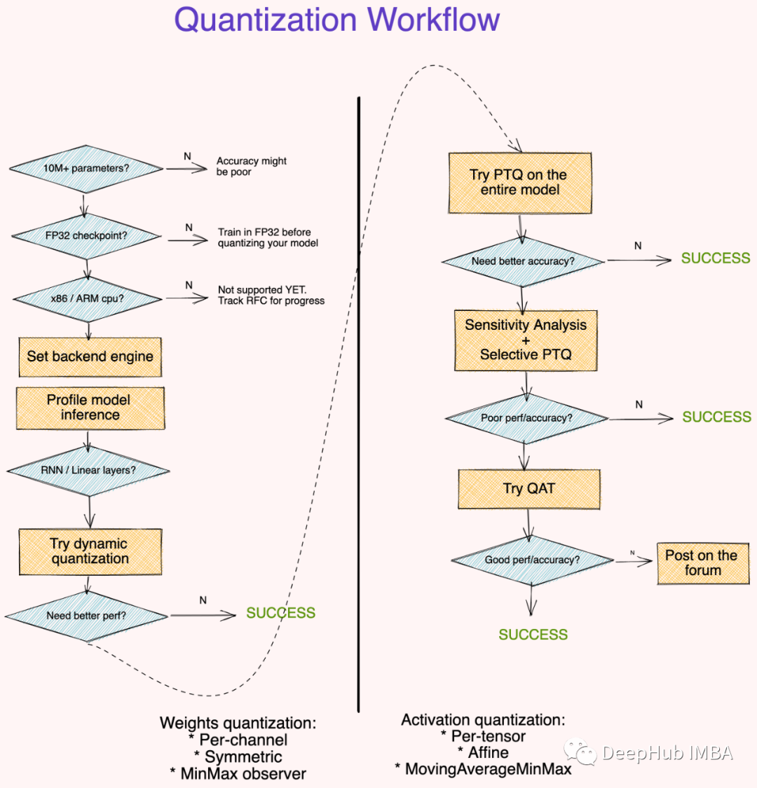
本文将使用CIFAR 10和一个自定义AlexNet模型，我对这个模型进行了小的修改以提高效率，最后就是因为模型和数据集都很小，所以CPU也可以跑起来。

import os
 import cv2
 import time
 import torch
 import numpy as np
 import torchvision
 from PIL import Image
 import torch.nn as nn
 import matplotlib.pyplot as plt
 from torchvision import transforms
 from torchvision import datasets, models, transforms
 
 device = "cpu"
 
 print(device)
 transform = transforms.Compose([
    transforms.Resize(224),
    transforms.ToTensor(),
    transforms.Normalize([0.485, 0.456, 0.406], [0.229, 0.224, 0.225])
    ])
 
 batch_size = 8
 
 trainset = torchvision.datasets.CIFAR10(root='./data', train=True,
                                        download=True, transform=transform)
 
 testset = torchvision.datasets.CIFAR10(root='./data', train=False,
                                        download=True, transform=transform)
 
 trainloader = torch.utils.data.DataLoader(trainset, batch_size=batch_size,
                                          shuffle=True, num_workers=2)
 
 testloader = torch.utils.data.DataLoader(testset, batch_size=batch_size,
                                          shuffle=False, num_workers=2)
 
 def print_model_size(mdl):
    torch.save(mdl.state_dict(), "tmp.pt")
    print("%.2f MB" %(os.path.getsize("tmp.pt")/1e6))
    os.remove('tmp.pt')

模型代码如下，使用AlexNet是因为他包含了我们日常用到的基本层：

from torch.nn import init
 class mAlexNet(nn.Module):
    def __init__(self, num_classes=2):
        super().__init__()
        self.input_channel = 3
        self.num_output = num_classes
         
        self.layer1 = nn.Sequential(
            nn.Conv2d(in_channels=self.input_channel, out_channels= 16, kernel_size= 11, stride= 4),
            nn.ReLU(inplace=True),
            nn.MaxPool2d(kernel_size=3, stride=2)
        )
        init.xavier_uniform_(self.layer1[0].weight,gain= nn.init.calculate_gain('conv2d'))
 
        self.layer2 = nn.Sequential(
            nn.Conv2d(in_channels= 16, out_channels= 20, kernel_size= 5, stride= 1),
            nn.ReLU(inplace=True),
            nn.MaxPool2d(kernel_size=3, stride=2)
        )
        init.xavier_uniform_(self.layer2[0].weight,gain= nn.init.calculate_gain('conv2d'))
 
        self.layer3 = nn.Sequential(
            nn.Conv2d(in_channels= 20, out_channels= 30, kernel_size= 3, stride= 1),
            nn.ReLU(inplace=True),
            nn.MaxPool2d(kernel_size=3, stride=2)
        )
        init.xavier_uniform_(self.layer3[0].weight,gain= nn.init.calculate_gain('conv2d'))
        
 
        self.layer4 = nn.Sequential(
            nn.Linear(30*3*3, out_features=48),
            nn.ReLU(inplace=True)
        )
        init.kaiming_normal_(self.layer4[0].weight, mode='fan_in', nnotallow='relu')
 
        self.layer5 = nn.Sequential(
            nn.Linear(in_features=48, out_features=self.num_output)
        )
        init.kaiming_normal_(self.layer5[0].weight, mode='fan_in', nnotallow='relu')
 
 
    def forward(self, x):
        x = self.layer1(x)
        x = self.layer2(x)
        x = self.layer3(x)
         
        # Squeezes or flattens the image, but keeps the batch dimension
        x = x.reshape(x.size(0), -1)
        x = self.layer4(x)
        logits= self.layer5(x)
        return logits
 
 model = mAlexNet(num_classes= 10).to(device)

现在让我们用基本精度模型做一个快速的训练循环来获得基线:

import torch.optim as optim 
 
 def train_model(model):
  criterion = nn.CrossEntropyLoss()
  optimizer = optim.SGD(model.parameters(), lr=0.001, momentum = 0.9)
 
  for epoch in range(2):
    running_loss =0.0
     
    for i, data in enumerate(trainloader,0):
       
      inputs, labels = data
      inputs, labels = inputs.to(device), labels.to(device)
 
      optimizer.zero_grad()
      outputs = model(inputs)
      loss = criterion(outputs, labels)
      loss.backward()
      optimizer.step()
 
      # print statistics
      running_loss += loss.item()
      if i % 1000 == 999:
        print(f'[Ep: {epoch + 1}, Step: {i + 1:5d}] loss: {running_loss / 2000:.3f}')
        running_loss = 0.0
   
  return model
 
 model = train_model(model)
 PATH = './float_model.pth'
 torch.save(model.state_dict(), PATH)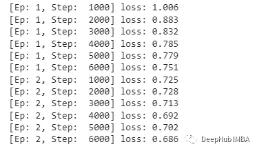

可以看到损失是在降低的，我们这里只演示量化，所以就训练了2轮，对于准确率我们只做对比。

我将做所有三种可能的量化:

1. 动态量化 Dynamic qunatization：使权重为整数(训练后)
2. 静态量化 Static quantization：使权值和激活值为整数(训练后)
3. 量化感知训练 Quantization aware training：以整数精度对模型进行训练

我们先从动态量化开始:

import torch
 from torch.ao.quantization import (
  get_default_qconfig_mapping,
  get_default_qat_qconfig_mapping,
  QConfigMapping,
 )
 import torch.ao.quantization.quantize_fx as quantize_fx
 import copy
 
 # Load float model
 model_fp = mAlexNet(num_classes= 10).to(device)
 model_fp.load_state_dict(torch.load("./float_model.pth", map_locatinotallow=device))
 
 # Copy model to qunatize
 model_to_quantize = copy.deepcopy(model_fp).to(device)
 model_to_quantize.eval()
 qconfig_mapping = QConfigMapping().set_global(torch.ao.quantization.default_dynamic_qconfig)
 
 # a tuple of one or more example inputs are needed to trace the model
 example_inputs = next(iter(trainloader))[0]
 
 # prepare
 model_prepared = quantize_fx.prepare_fx(model_to_quantize, qconfig_mapping, 
                  example_inputs)
 # no calibration needed when we only have dynamic/weight_only quantization
 # quantize
 model_quantized_dynamic = quantize_fx.convert_fx(model_prepared)

正如你所看到的，只需要通过模型传递一个示例输入来校准量化层，所以代码十分简单，看看我们的模型对比：

print_model_size(model)
 print_model_size(model_quantized_dynamic)

可以看到的，减少了0.03 MB或者说模型变为了原来的75%，我们可以通过静态模式量化使其更小:

model_to_quantize = copy.deepcopy(model_fp)
 qconfig_mapping = get_default_qconfig_mapping("qnnpack")
 model_to_quantize.eval()
 # prepare
 model_prepared = quantize_fx.prepare_fx(model_to_quantize, qconfig_mapping, example_inputs)
 # calibrate 
 with torch.no_grad():
    for i in range(20):
        batch = next(iter(trainloader))[0]
        output = model_prepared(batch.to(device))

静态量化与动态量化是非常相似的，我们只需要传递更多批次的数据来更好地校准模型。

让我们看看这些步骤是如何影响模型的:

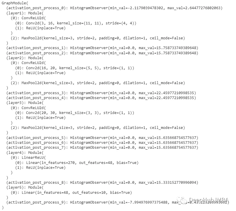
可以看到其实程序为我们做了很多事情，所以我们才可以专注于功能而不是具体的实现，通过以上的准备，我们可以进行最后的量化了：

# quantize
 model_quantized_static = quantize_fx.convert_fx(model_prepared)

量化后的model_quantized_static看起来像这样:

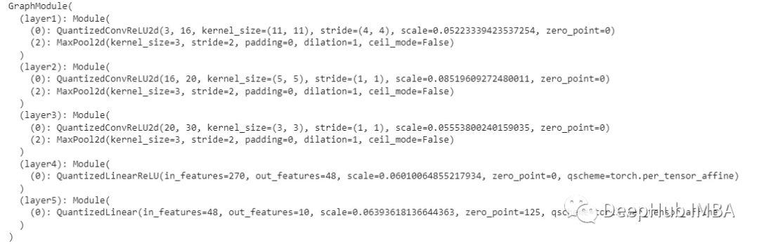
现在可以更清楚地看到，将Conv2d和Relu层融合并替换为相应的量子化对应层，并对其进行校准。可以将这些模型与最初的模型进行比较:

print_model_size(model)
 print_model_size(model_quantized_dynamic)
 print_model_size(model_quantized_static)

量子化后的模型比原来的模型小3倍，这对于大模型来说非常重要

现在让我们看看如何在量化的情况下训练模型，量化感知的训练就需要在训练的时候加入量化的操作，代码如下：

model_to_quantize = mAlexNet(num_classes= 10).to(device)
 qconfig_mapping = get_default_qat_qconfig_mapping("qnnpack")
 model_to_quantize.train()
 # prepare
 model_prepared = quantize_fx.prepare_qat_fx(model_to_quantize, qconfig_mapping, example_inputs)
 
 # training loop 
 model_trained_prepared = train_model(model_prepared)
 
 # quantize
 model_quantized_trained = quantize_fx.convert_fx(model_trained_prepared)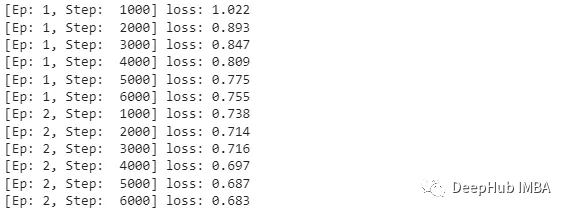

让我们比较一下到目前为止所有模型的大小。

print("Regular floating point model: " )
 print_model_size( model_fp)
 print("Weights only qunatization: ")
 print_model_size( model_quantized_dynamic)
 print("Weights/Activations only qunatization: ")
 print_model_size(model_quantized_static)
 print("Qunatization aware trained: ")
 print_model_size(model_quantized_trained)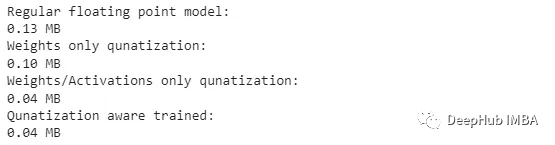

量化感知的训练对模型的大小没有任何影响，但它能提高准确率吗?

def get_accuracy(model):
  correct = 0
  total = 0
  with torch.no_grad():
      for data in testloader:
          images, labels = data
          images, labels = images, labels
          outputs = model(images)
          _, predicted = torch.max(outputs.data, 1)
          total += labels.size(0)
          correct += (predicted == labels).sum().item()
 
      return 100 * correct / total
 
 fp_model_acc = get_accuracy(model)
 dy_model_acc = get_accuracy(model_quantized_dynamic)
 static_model_acc = get_accuracy(model_quantized_static)
 q_trained_model_acc = get_accuracy(model_quantized_trained)
 
 
 print("Acc on fp_model:" ,fp_model_acc)
 print("Acc weigths only quantization:", dy_model_acc)
 print("Acc weigths/activations quantization" ,static_model_acc)
 print("Acc on qunatization awere trained model:" ,q_trained_model_acc)

为了更方便的比较，我们可视化一下：

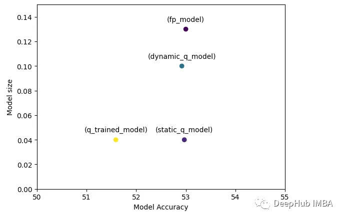
可以看到基础模型与量化模型具有相似的准确性，但模型尺寸大大减小，这在我们希望将其部署到服务器或低功耗设备上时至关重要。